A dissertation submitted in partial fulfilment of the requirements for the degree of Master of Science (MSc) in Marine Biology. School of Ocean Sciences, Bangor University. Submitted 31 January 2019.
Reproduced as submitted, minus the university declaration pages, with typographic corrections and one dead link removed. I came back to this subject years later with global data in the Protected Mangroves Dashboard.
Abstract
Indonesia holds the greatest proportion of the world’s mangrove forests. Mangroves provide multiple ecosystem services such as protection from natural disasters, enhancing fisheries, the provision of timber and store a high density of carbon. Despite their importance, they have suffered rapid deforestation across the globe, particularly in Indonesia. Global efforts to protect tropical forests are usually centred on the establishment of protected areas (PAs). However, their effectiveness has been challenged in recent years as PAs are often allocated to remote and inaccessible regions that would face low rates of deforestation anyway. Furthermore, because of this remoteness bias, conventional methods of assessing PA effectiveness often overestimate the protection they provide. For this study, a recent high-resolution mangrove map was produced (at 30 m resolution). This was used to map nationwide mangrove deforestation between the year 2000 to 2017. The effectiveness of Indonesian PAs at preventing mangrove deforestation was then quantified using matched sampling techniques. Results from this study confirm that Indonesian PAs are generally located in remote inaccessible regions, and that this bias does indeed lead to overestimates in PA effectiveness when using conventional inside-out comparisons. The results of matching estimate Indonesian PAs prevented the loss of 3.5% of protected mangroves. Furthermore, Strict Nature Reserves (SNRs), which specifically focus on preserving biodiversity, were found to be ineffective at preventing mangrove deforestation. These results show that Indonesian PAs are slightly effective at preventing the deforestation of mangroves. However, despite this small effect, habitat destruction within Indonesian PAs continues to be of concern. The Indonesian government needs to focus on increasing efforts on enforcing protection from illegal logging activities within PA boundaries, particularly of SNRs, if they are to preserve their mangroves for future generations.
1. Introduction
In the year 2000, Indonesia’s coastline held over 20% of all the world’s mangrove forests; equal to approximately 3 million ha (Spalding, Kainuma and Collins, 2010; Giri et al., 2011). Southeast Asia is a global hotspot for mangrove diversity, with over 268 plant species recorded to live amongst mangrove vegetation; 52 of which are considered ’true’ mangroves. All of these species can be found within Indonesian borders (Giesen et al., 2007; Spalding, Kainuma and Collins, 2010). Worldwide, mangroves are thought to provide up to US$1.6 billion in ecosystems services per year and are a vital commodity to many coastal communities (Costanza et al., 1997; Polidoro et al., 2010). They provide a wealth of natural resources and ecosystem services such as the protection of coastlines from tropical storms and tsunamis, support of local and regional fisheries to the provision of wood or timber for shelter and construction (Spalding, Kainuma and Collins, 2010). Not only do these services contribute to global or regional economies, they serve to benefit local or indigenous people, many of whom are poor or have a low-impact sustainable relationship with mangroves (Osti, Tanaka and Tokioka, 2009). Furthermore, mangroves play a vital global role in the storage and sequestration of carbon, which is of increasing international importance towards the mitigation of global climate change (Donato et al., 2011).
Indonesia’s mangrove forests suffered severe decline throughout much the 20th century. Islands such as Java and Sulawesi, where human population faced rapid expansion over the past 5 decades, saw declines of up to 70% of their original mangrove area (Ilman et al., 2016). This was primarily to make way for the construction of urban landscapes or shrimp farms (Richards and Friess, 2016). Deforestation at this scale has had a negative impact on the biodiversity of mangrove forests, with 16% of species now threatened by extinction (Polidoro et al., 2010; Richards and Friess, 2016).
Reducing global deforestation to preserve biodiversity and mitigate or reverse climate change is becoming a matter of increasing urgency for many governments worldwide, especially since the direct and indirect ecosystem services they provide are becoming more realised. Governments often consider the establishment of protected areas (PAs), along with the restriction of human activity within PAs as the most effective strategy at reducing deforestation and habitat destruction (Chape et al., 2005; Miteva, Murray and Pattanayak, 2015).
Despite international efforts to preserve biological diversity of tropical forests (including mangroves), many protected areas have suffered continued deforestation within their boundaries. This is especially true for PAs across Indonesia, where some regions have lost more than 50% of their lowland tropical forests since the 1980s (Curran et al., 2004). This has raised many questions within scientific, legal and environmental activist groups as to the effectiveness of PAs at preventing tropical deforestation (Andam et al., 2008). It is often reported that PAs are understaffed or staffed by underpaid rangers whom may be prone to corruption (Watson et al., 2014; Wright et al., 2007), park boundaries may be inadequately demarcated or ineffectively managed by local authorities, and leaders tend to favour economically profitable practices that focus on resource extraction rather than conservation (Gaveau et al., 2009). Additionally, the establishment of a PA can cause the displacement of deforestation to neighbouring unprotected regions through the relocation of indigenous people, or the attraction of migrants and logging industries to these adjacent lands (Wittemyer et al., 2008).
Objectively measuring the effectiveness of conservation strategies such as the establishment of PAs is of great importance for both the preservation of biological diversity, and for the protection of the rights of people who inhabit these regions (Springer, Campese and Painter, 2011). Historically, simple inside-out comparisons have driven the conclusion that PAs are effective at protecting tropical forests (Bruner et al., 2001; Naughton-Treves, Holland and Brandon, 2005; Joppa, Loarie and Pimm, 2008). However, this notion has been challenged by recent literature (e.g. Andam et al., 2008; Gaveau et al., 2009), as this simple inside-out comparison fails to take into account the geographical location of PAs, leading researchers or policymakers to overestimate the true effectiveness protection actually provides. Inside-out comparisons ignore the fact that PAs are often established in remote or inaccessible locations that would have unlikely faced deforestation anyway, even in the absence of protection (e.g. Andam et al., 2008; Gaveau et al., 2009; Joppa and Pfaff, 2009; Miteva, Murray and Pattanayak, 2015). Moreover, people tend to respond to the allocation of a PA by relocating to neighbouring regions, thus displacing deforestation to outside the PA boundary. This would make a network of PAs appear more effective at reducing deforestation than they actually are. (Andam et al., 2008; Wittemyer et al., 2008).
These issues have led researchers to use more novel approaches when assessing the effectiveness of PAs at protecting biological diversity. A recent study measuring the effectiveness of PAs at reducing rainforest deforestation in Costa Rica found that measurement accuracy could be substantially improved by controlling for a set of observable spatial biases known to impact rates of tropical deforestation (Andam et al., 2008). By controlling for these confounding variables, they were able to accurately determine how much rainforest avoided deforestation as a result of protection. They also found that failing to observe for these spatial biases substantially increased their estimate of prevented deforestation.
This leads to the primary objective of the present study: How effective are PAs at preventing the deforestation of mangrove forests? Several aspects of this question will be investigated by measuring the effectiveness of Indonesia’s protected area network at preserving mangrove forests. Indonesia was chosen to explore this question as it holds a substantial portion of the world’s mangroves (>20%) and has suffered severe deforestation over the past several decades. This will be achieved by: (1) calculating mangrove deforestation over the past 2 decades by the production of an up-to-date, high-resolution mangrove map for the whole of Indonesia; (2) quantifying the remoteness of Indonesian PAs and how this spatial bias can influence measurement accuracy; (3) estimating the area of mangroves that avoided deforestation directly as a result of protection efforts; and (4), to determine if the ‘strictness’ of PA protection impacts rates of mangrove deforestation.
2. Materials and Methods
2.1. Mapping Mangrove Deforestation
In order to determine the rate and extent of mangrove deforestation across Indonesia for the past two decades, data on mangrove forest loss was needed. This data was obtained from two publicly available high-resolution datasets (in raster format): The Global Mangrove Distribution (GMD) layer (Giri et al., 2011), and the Global Forest Change (GFC) dataset (v1.5) (Hansen et al., 2013). Both datasets were processed from Landsat 7 imagery at a resolution of roughly 30 m (0.09 ha) per pixel.
The GMD and GFC are both continuous, globally consistent forest-cover datasets. They are easily comparable with one another as both were computed from imagery captured by the same satellite, thus have the same resolution. The GMD is only available for the year 2000, however, this allowed for the identification of areas with mangrove forest in Indonesia for the year 2000, forming the baseline of the analysis. The GFC dataset does not identify forest type, it includes global forest cover for the year 2000 and 2017. It also identifies per-pixel forest loss for each year from the year 2000 until 2017.
In order to produce an updated mangrove map for the year 2017, the forest loss pixels from the GFC dataset were used to identify and mask out (remove) pixels from the GMD dataset (Figure 1). As previously stated, the GMD represents the global extent of mangroves for the year 2000. The GFC identifies annual forest change for all forests (including mangroves, however it doesn’t distinguish forest type) from the year 2000. In this instance, the GFC was used to estimate the current state of mangrove forests by using the regions of deforestation they identified in their dataset to remove pixels in the GDM layer. This gave a mangrove cover map of Indonesia for the present day at 30 m resolution.
This served to provide three sources of information for geospatial statistical analysis: (1) baseline mangrove cover for the year 2000; (2) estimated updated mangrove cover for the year 2017; and (3) mangrove loss between 2000 and 2017 (i.e. the difference between 1 and 2).

Figure 1. Flow chart to visualise method used for obtaining mangrove datasets for analysis.
The Google Earth Engine (GEE) cloud computing platform was used to conduct the imagery analysis for this study. There are several benefits to using GEE over more traditional GIS software. Namely, GEE is completely free to use, and is relatively easy to access by signing up for an account here https://earthengine.google.com. In addition to this, many publicly available datasets and satellite imagery are provided in their catalogue and can be easily accessed using the native search feature within the GEE platform. Furthermore, it works very well for large image files as they are always stored on the GEE servers and processing is done in parallel by mapping the computation across thousands of CPUs on many different servers simultaneously. This offers an enormous speed advantage.
It would be possible to use a similar method to estimate mangrove forest gain as the GFC dataset includes global forest gain as a separate layer. However, only deforestation was considered for this study as forest gain does not serve to answer the hypothesis, which centres around reduction in forest cover as a response to protection rather than net change.
2.2. Protected Areas
Geospatial data on Indonesian PA boundaries was obtained from the World Database on Protected Areas (WDPA) (UNEP-WCMC and IUCN, 2019) as a GIS shapefile. In the 2018 version, there were 733 reported PAs for Indonesia. This shapefile included an attribute table which contained metadata on the PA features. This information was used to recombine fields in preparation for analysis.
It was decided that PAs should not be omitted based on the date in their ‘Status Year’ field. The WDPA user manual (WDPA, 2017) states that this field is used to identify the year the current designation status was set. So, if the PA designation status was changed from ‘Proposed’ to ‘Designated’ in 2006, then the value in ‘Status Year’ would be ‘2006’ indicating when this change occurred. The date does not refer to when a geographical space was first protected. Additionally, the majority of the ‘Status Year’ fields were missing a date for Indonesia’s PAs, so to omit all of these would have a significant impact on the analysis. Therefore, it was decided to include all PAs regardless of the reported date. This assumption may cause some issues where PAs were only recently designated, however, even with a few years of protection, there would still likely be a small measurable impact on mangrove deforestation. Often, sites benefit from protection several years before official designation anyway (WDPA, 2017).
There are 6 IUCN protected area categories. The IUCN developed this system to classify, record and define the wide variety of management aims and objectives PAs across the globe typically have (IUCN, 2008). Broadly speaking, the first two categories (Ia, Ib and II) include national parks and biosphere reserves and are primarily focused on strict habitat protection where public visitation, human intervention or resource extraction are strictly prohibited. Whereas, the other categories (III – VI) target the preservation of specific species, habitats or inhabited landscapes which require continued management and monitoring and may allow for some form of limited resource extraction. For the sake of the present study, the 6 IUCN categories were recombined into three groups for testing. This was done to determine if ‘strictness’ of protection influences deforestation. IUCN categories Ia, Ib and II and were labelled the Strict Nature Reserves (SNRs). This group reflects PAs that are typically uninhabited regions where any form of (legal) habitat alteration should be minimal. The second group included the other categories (III – VI) and were labelled the Species Management Reserves (SMRs). This groups reflects PAs where human intervention and habitat alteration are expected as they require continued management and monitoring. Finally, the fields where the IUCN category was ‘Not Reported’ were combined into their own group (the WDPA user manual recommends this) and were labelled the Not Reported Reserves (NRRs) (Figure 2).
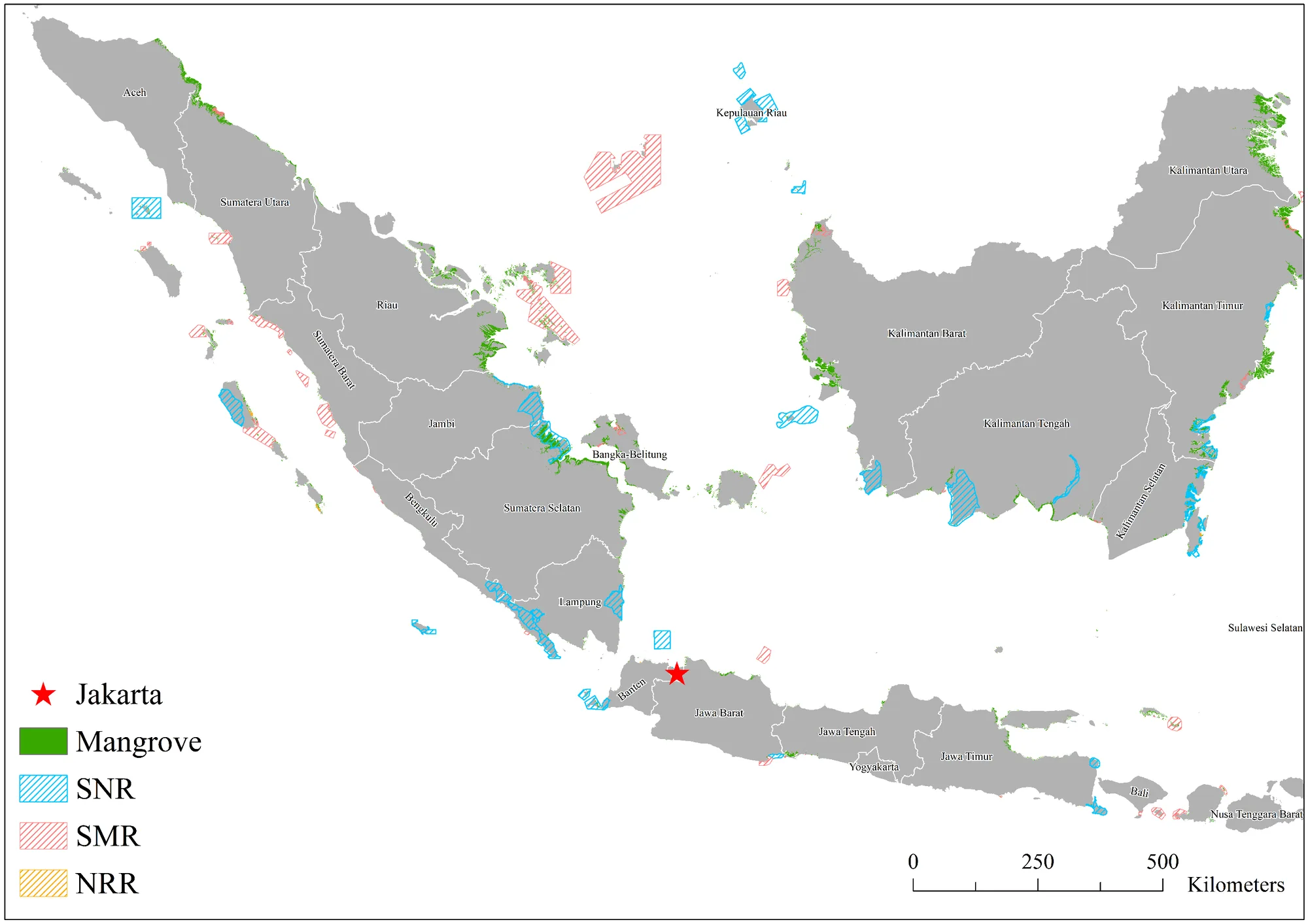
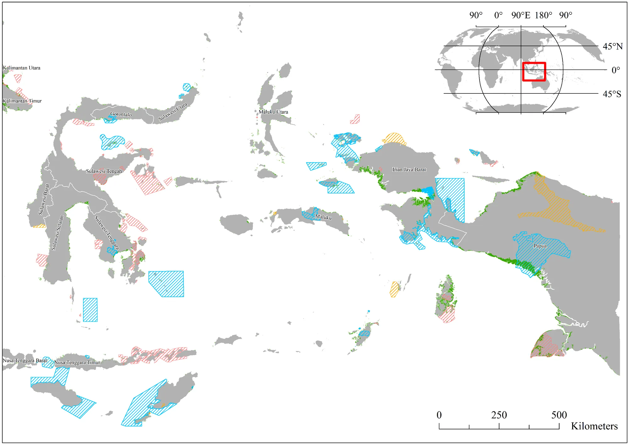
Figure 2. Distribution of Indonesia’s mangrove forests for the year 2000 and PAs that intersected mangroves in the year 2017. SNR = Strict Nature Reserves (IUCN categories Ia, Ib and II), SMR = Species Management Reserves (IUCN categories III – VI), and NRR = Not Reported. Western Indonesia is shown above, eastern Indonesia below.
2.3. Sampling strategy
Sampling was done in ArcMap 10 as GEE is not suitable for handling the computation of large vector feature-sets. A random sample of 5,000 plots were scattered across the entire of Indonesia’s mangrove forests in the year 2000. Each plot had an area of roughly 500 m² (25 ha), making the total sample area 125,000 ha. Plots were placed at a minimum of 1 km from one another to minimise the effects of spatial-autocorrelation (Stewart Fotheringham and Rogerson, 1993). In the year 2000, Indonesia had about 3 million ha of mangrove forests, and the samples cover roughly 85,885 ha of this – representing 0.03% of Indonesia’s mangroves. This strategy was used to ensure an even spread of plots across the whole country and ensured the plots fell entirely within the baseline mangrove region (i.e. portions of the plots did not hang outside of the mangrove region). Similar studies conducted on large inland forests typically use much larger plots (e.g. Gaveau et al., (2009) used 1,264 plots at 2,500 ha). This strategy might not be appropriate for analysing mangroves within protected areas, as plots that size would be much larger than many of the PAs thus meaning smaller PAs would need to be excluded from the analysis. Additionally, significant portions of the plots would hang outside of the study region as mangroves are usually only found along a thin strip of the coastline (typically no thicker than 10 km). Furthermore, much larger plots would be incapable of accurately representing the finer resolution of the covariate data, as important regional variations across these greater distances (for example population density) would be missed at this scale. After the samples were drawn, 372 plots were excluded as they fell on the boundary of protected areas, and 88 plots were excluded as they fell within 1 km of another plot thus giving a total of 4,540 plots for the analysis.
The samples were layered over the three mangrove maps described in Section 3.2, and the covariate datasets (explained in Section 3.7). Sample data was extracted using the zonal statistics tool in ArcMap. This gave each of the 4,540 plots a value for mangrove cover for both years 2000 and 2017, mangrove loss between this period (i.e. the difference between the two) and a value for each of the covariate datasets.
2.4. Response variables
Percent deforestation was the response variable for this study. This was calculated for each plot by dividing the number of deforested pixels by the number of forested pixels from the baseline year (the year 2000). This gave values on a continuous scale that ranged from 0 to 100% where 0% equals no deforestation and 100% equals total deforestation (i.e. no pixels remained from the baseline) (Laurance et al., 2002).
2.5. Matched sampling
To answer the question ‘how effective are PAs at preventing the deforestation of mangrove forests?’ we first need to ascertain what would have happened to mangrove forests within plots had they never been protected in the first place. There are difficulties with estimating this counterfactual outcome as it is not possible to observe the outcome of a plot had it not been protected in the first place. One could try to compare the outcome of protected plots with that of nearby unprotected plots, then use this difference as an estimate of the PA effectiveness (Mas, 2005; Joppa, Loarie and Pimm, 2008). However, there are several issues with this method. As stated before, PAs are often placed in non-random locations. It is common for policy-makers to designate protected areas in remote, inaccessible regions that are unlikely to face deforestation anyway (Venter et al., 2018). Therefore, an inside-out comparison would be biased, and not a good indication of how that region would have fared in the absence of protection.
Another method could be through the use of a parametric regression analysis (Cropper, Puri and Griffiths, 2001), whilst factoring confounding variables known to impact rates of tropical deforestation. The issue with this approach is that variations in the distribution of covariate data between the treatment and control groups can severely increase statistical bias (Cochran and Rubin, 1961; Imbens and Wooldridge, 2008).
Therefore, a method that makes as few parametric assumptions as possible (Rosenbaum and Rubin, 1985), and avoids simple inside-out comparisons is preferred. Matched sampling is a non-parametric multivariate technique that can be used to assess what may have occurred if a treatment (i.e. the establishment of a PA) had not been applied. This is achieved by selecting sample units from a large pool of potential controls (i.e. unprotected samples) to produce a new control group that is similar in size and distribution of observed covariates to the treated group (Rosenbaum and Rubin, 1985). Therefore, individual protected samples are matched to individual unprotected samples based on their similar spatial and socio-economic characteristics. This method essentially mimics a randomised control trial – whereby the treated and control groups are both as similar as possible (except for the treatment they receive), therefore, any differences in outcomes are likely a result of the treatment they received (Ferraro and Hanauer, 2014).
2.6. Average Treatment Effect on the Treated (ATT)
After matching, the new dataset can then be used to quantify the amount of mangrove forests that avoided deforestation due to protection. This can be quantified by estimating the ATT which measures the causal effect of treatment (i.e. protection) on the outcome (i.e. deforestation). The following section will explain how this works:
The Neyman-Rubin theory of causal inference (Rubin, 1973; Splawa-Neyman, 1990) is a framework that can be used to model this type of problem. The model assumes each unit has two potential outcomes – i.e. one if the unit was treated, and the other if the unit had never received treatment. The notation of the model is widely used in the literature and provides a useful way to demonstrate the theory (Sekhon, 2007). The units (i.e. the sample plots) for this study - denoted as i - either fell within protected or unprotected regions – or in words used to describe the model they were either treated (Ti = 1) or untreated (Ti = 0) respectively. The outcome of interest (Y) is the response variable (or % deforestation). Therefore, Yi1 denotes the outcome if the unit was treated, and Yi0 denotes the outcome if the unit was not treated. These are the observed potential outcomes and are used to estimate the treatment effect on each unit i. This is important, because when attempting to measure the effectiveness of a treatment on a population, one needs to know - for each unit - what the outcome would have been if the unit had never received treatment in the first place.
Therefore, when considering mangrove deforestation within PAs, each plot needs to have an observed treated outcome Yi1 and an expected outcome Yi0 (as if the plot had never been protected). From this, the treatment effect for each of the treated units can be estimated, then used to calculate the Average Treatment Effect on the Treated (ATT), which can be summarised by the following formula:
In the case of quantifying the effect of protection at preventing mangrove deforestation, the ATT would be the sum of observed percent deforestation Yi1 minus the expected percent deforestation Yi0 (i.e. if the plot had not been protected) divided by all of the protected plots (Ti = 1).
The obvious issue here is that the potential outcomes Yi1 and Yi0 are jointly unobservable, i.e. only one outcome can be observed for each unit. (Ho et al., 2011; Flores and Chen, 2018). It would not be possible to know how protected plots would have fared had they not been protected in the first place. As explained previously, matching methods are a way to attain a control group that has been selected by the matching algorithm to be as similar to the treated group as possible. The expected outcomes Yi0 for the treated group (Ti = 1) can be estimated by fitting a model to the matched data to create a set of simulated Yi0 values for the treated units. The model essentially predicts the expected value of the outcome variable among the treated units as if the treated units were control units (Ho et al., 2011).
For the present study, the MatchIt package in R was used. Treated samples were matched to comparable untreated samples using propensity score matching on the covariates (Sekhon, 2008). The propensity score is a distance measure calculated for each unit based on a logistic regression model of the covariates. Pairs from the treated and control groups were matched based on their propensity score using the nearest-neighbour algorithm with a caliper size of 0.2; this ensured only closely matched pairs were included (Cochran and Rubin, 1961; Rosenbaum and Rubin, 1985; Andam et al., 2008).
Post-matching performance was evaluated from the balance tables by comparing differences in covariate means between treated and control groups before and after matching to see if the differences had been eliminated. The balance tables were also used to assess the remoteness of protected areas compared to the wider Indonesian landscape.
After matching, the ATT for the treated units was estimated using the Zelig package in R. A model-based method was applied to predict the expected outcome for each plot. This was done by fitting a linear least-squares model to the observed outcomes for the matched data (Imai, King and Lau, 2007), therefore giving an observed Yi1 and simulated Yi0 value for each plot. ATT was then calculated using Formula 1, along with 95% confidence interval to indicate significance. The final output is a value that estimates the percentage of mangrove deforestation that was avoided within Indonesian protected areas over the past two decades. A negative value indicates a causal link between protection status and avoided deforestation independent from the covariates (Andam et al., 2008). Matching was performed three times: (1) for treated plots from all PAs paired with unprotected control plots; (2) for treated plots from only Strict Nature Reserves (SNRs) paired with unprotected control plots; and (3) treated plots from Species Management Reserves (SMR) paired with unprotected control plots. Not Reported Reserves (NRRs) were not included due to the small number of samples.
2.7. Confounding variables
Matching models can only be as good as the included observable covariates. A handful of core variables that are known to impact rates of tropical deforestation and PA placement were used. These confounders were selected based on recommendations in the current literature (e.g. Laurance et al., 2002; Andam et al., 2008; Gaveau et al., 2009), and accessibility of the data (they had to be free and open access). Specifically, the covariate data included: proximity to potential markets (i.e. distance to ports, distance to highways, distance to major cities), landcover characteristics (proximity to forest edge, accessibility to urban areas), and socioeconomic data such as regional population density and regional levels of poverty. An overview of the covariate data used can be seen in Table 1.
Table 1. Covariate datasets and units used for propensity score matching. These variables are known to impact rate of tropical deforestation.
| Code | Covariate (units) | Reference |
|---|---|---|
| popd | District level population density (ppl/km²) | Gaughan et al., 2013 |
| povd | District level people in poverty (%) | PODES Indonesia |
| fte | Distance to forest edge (m) | my data |
| acc | Accessibility to cities (minutes) | Weiss et al., 2018 |
| ctd | Distance to nearest district capital city (m) | my data |
| rds | Distance to nearest highway (m) | my data |
| prt | Distance to nearest port (m) | my data |
Distance to ports, highways, major cities and forest edge were calculated as separate rasters using the cumulative cost function in GEE. This calculated - per pixel – the cumulative Euclidean distance in metres from the source. This was done for the entire of Indonesia.
The accessibility to cities dataset quantifies travel time to the nearest city for 2015 (Weiss et al., 2018). This dataset uses a friction map that takes into account landcover characteristics, water bodies, topographical conditions, railways, roads and road attributes.
District level population density was calculated from the Asia population count raster provided on the WorldPop website (www.worldpop.org.uk). The raster gives population count per 100m pixels for the whole of Southeast Asia for 2010 (Gaughan et al., 2013). Using a shapefile of Indonesia’s administrative areas (obtained from GADM – www.gadm.org), this raster was used to calculate the population of each Indonesian district using the zonal statistics tool in ArcMap 10. Population density was estimated by dividing district population by district area.
Socioeconomic data was obtained from PODES (Village Potential Statistics – Indonesia). The Foster-Greer-Thorbecke (FGT) index was used for each Indonesian district. The FGT index is a calculation that indicates the proportion of people who live below the poverty line. A value of 25 percent indicates 25 people out of 100 are considered poor. More information can be found here (http://povertymap.smeru.or.id/indicators-explained).
3. Results
3.1. Mangrove deforestation patterns across Indonesia over the past two decades
The results in Table 2 give the summary statistics of Indonesian mangrove deforestation between 2000 and 2017. They show Indonesia contained 2.72 million hectares of mangrove forest in the year 2000. However, 320,000 ha was deforested by 2017. This is a rate of roughly 0.7% per year; which is comparable to previous estimates of mangrove loss for Indonesia (Gaughan et al., 2013; Murdiyarso et al., 2015). On the other hand, deforestation within protected areas was much lower, at a rate of about 0.3% per year. Figure 3 shows the distribution and extent of mangrove deforestation across Indonesia. Note some of the cells - especially across the islands of Java and Sulawesi – have lost > 80% of their mangrove forests since the year 2000.
Table 2. Summary statistics on the state of Indonesian mangroves between 2000 and 2017 and an inside-out comparison of deforestation rates for Indonesian PAs. The SNR, SMR and NRR columns are IUCN groups: SNR = strict nature reserves, SMR = species management reserves and NRR = not reported. Deforestation is calculated as (forest loss)/(forest cover in 2000) * (100).
| Indonesia | All PAs | SNR | SMR | NRR | |
|---|---|---|---|---|---|
| Forest cover in 2000 (ha) | 2,717,863 | 653,374 | 472,380 | 166,886 | 14,108 |
| Forest cover in 2017 (ha) | 2,396,185 | 617,965 | 443,672 | 160,440 | 13,854 |
| Forest loss 2000 - 2017 (ha) | 321,678 | 35,409 | 28,708 | 6,446 | 254 |
| Deforestation (%) | 11.83 | 5.42 | 6.08 | 3.86 | 1.80 |
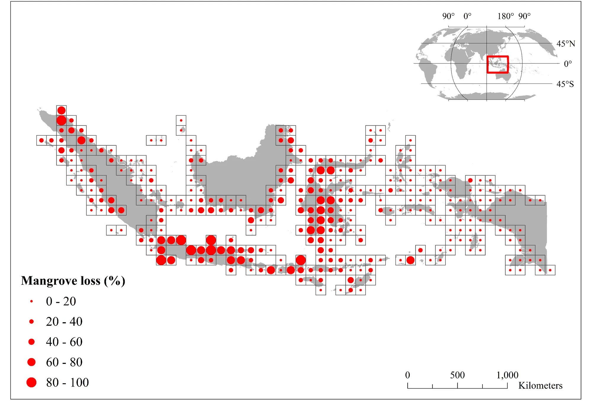
Figure 3. Distribution of mangrove deforestation across Indonesia between the years 2000 – 2017. Each cell represents 100 km². The red dots signify percent mangrove forest lost for each cell. The densely populated islands of Java and Sulawesi have suffered the greatest mangrove deforestation.
3.2. Controlling for bias
The results in Table 3 show the output from covariate balancing. These results assess the differences in covariate means between protected and unprotected plots before and after matching. The third and fourth columns in Table 3 present the mean covariate values for unprotected and protected plots before matching, and the fifth and sixth columns show the covariate means after matching. The seventh column shows percent difference (i.e. how much the matching improved balance) in means after matching. For example, before matching, the first row (population density for all PAs) shows mean population density is much lower for protected plots (23 people per square kilometre) compared to unprotected plots (92 people per square kilometre). However, after matching this was improved by 98.5%. This indicated a very good match for this covariate. Similar results can be seen for the other covariates. These figures demonstrate the remoteness and inaccessibility of PAs in Indonesia. There was a clear difference in covariate means between protected and unprotected lands before matching. Protected plots appeared to be located in sparsely populated regions that were less accessible to cities, roads and ports. Interestingly, mean distance to forest edge was considerably higher in protected regions, indicating PAs also tend to be located in deep forest. Therefore, propensity score matching has successfully balanced the confounding variables. This means that any difference in rates of deforestation between the treated and control groups can be exclusively attributed to the protection status of the plot.
Table 3. Covariate balance table for pre- and post-matched plots. The means for the unmatched groups have a greater difference than the matched groups indicating good balance of the covariates. % Diff = the percent improvement of the matched groups from the unmatched groups. SNR = Strict Nature Reserves, and SMR = Species Management Reserves.
| Covariate | IUCN type | Unmatched control mean | Unmatched treated mean | Matched control mean | Matched treated mean | % Diff. |
|---|---|---|---|---|---|---|
| Population density (km²) | All | 92 | 23 | 29 | 28 | 98.50 |
| SNR | 92 | 26 | 38 | 31 | 88.38 | |
| SMR | 92 | 16 | 49 | 41 | 89.33 | |
| Poverty (%) | All | 42 | 39 | 41 | 42 | 88.40 |
| SNR | 42 | 41 | 43 | 42 | 75.86 | |
| SMR | 42 | 29 | 36 | 33 | 78.19 | |
| Forest edge (m) | All | 163 | 416 | 277 | 287 | 95.69 |
| SNR | 163 | 503 | 300 | 306 | 98.06 | |
| SMR | 163 | 213 | 193 | 192 | 99.55 | |
| Accessibility to cities (minutes) | All | 404 | 700 | 536 | 554 | 94.02 |
| SNR | 404 | 611 | 556 | 541 | 93.11 | |
| SMR | 404 | 928 | 390 | 261 | 75.44 | |
| Distance to cities (m) | All | 47,550 | 92,031 | 68,944 | 66,900 | 95.40 |
| SNR | 47,550 | 61,446 | 60,345 | 58,053 | 83.51 | |
| SMR | 47,550 | 172,854 | 67,165 | 63,862 | 97.36 | |
| Distance to roads (m) | All | 46,607 | 91,316 | 60,259 | 62,349 | 95.33 |
| SNR | 46,607 | 56,854 | 54,122 | 53,435 | 93.29 | |
| SMR | 46,607 | 181,671 | 53,961 | 36,779 | 87.28 | |
| Distance to ports (m) | All | 94,216 | 110,269 | 90,151 | 84,265 | 63.33 |
| SNR | 94,216 | 67,494 | 76,037 | 69,561 | 75.76 | |
| SMR | 94,216 | 215,765 | 117,811 | 98,891 | 84.43 | |
| Number of samples (n) | All | 3636 | 904 | 683 | 683 | - |
| SNR | 3636 | 639 | 508 | 508 | - | |
| SMR | 3636 | 244 | 75 | 75 | - |
Figure 4 shows mean deforestation rates of the sample dataset within and outside of PAs both before and after matching. Mean deforestation was about 50% greater before matching, indicating that not controlling for covariate bias overestimates PA effectiveness. After matching, deforestation rate between unprotected and protected plots was significantly different (t = 3.25, df = 1328.8, P = <0.001), indicating that - even after balancing - Indonesian PAs still have a statistically significant impact on preventing mangrove deforestation.
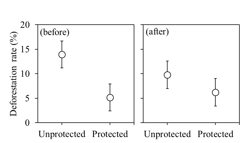
Figure 4. Comparison of mean deforestation rates before and after matching for all Indonesian PAs between 2000 to 2017. Error bars indicate 95% CI.
3.3. Avoided deforestation and PA ‘strictness’
Figure 5 shows the ATT results from the propensity score matching analysis. The Not Reported Reserves (NRRs) were omitted due to the very small sample size. The ATT indicates the overall percentage increase or decrease of the response variable as a result of the treatment. Thus, a negative value would indicate avoided deforestation as a direct result of protection. These results imply that Indonesian PAs have a small but statistically significant impact on preventing mangrove deforestation. All PAs prevented the deforestation of approximately 3.5% of Indonesia’s mangrove forests. This equates to approximately 22,704 ha of protected mangroves that avoided deforestation between the year 2000 and 2017 as a direct result of protection. Most of this protection was accounted for by mangroves in SMRs, as SNRs did not have a significant impact on deforestation (Figure 5).
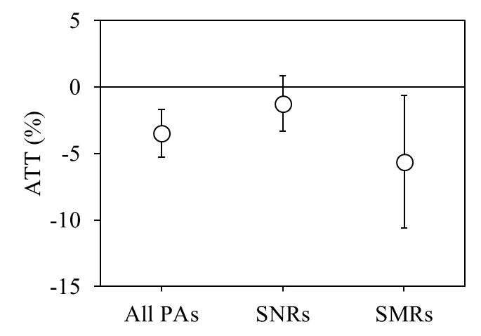
Figure 5. ATT outputs from the matching analysis estimating PA impact on mangrove deforestation. Negative values indicate reduction in PA deforestation as a result of protection. Error bars indicate 90% confidence interval. Values are statistically significant if error bar does not cross zero. SNR = Strict Nature Reserves; SMR = Species Management Reserve
4. Discussion
Results from this study offer a more reliable estimation of PA performance than more conventional inside-out comparisons. Through the development of an up-to-date, highresolution mangrove map of Indonesia, and by controlling for PA remoteness, results from this study demonstrate that PAs in Indonesia have at least partially prevented the deforestation of mangroves over the past two decades. Initially, the results in Table 2 and Figure 4 (before) show Indonesian PAs had much lower rates of mangrove deforestation compared to the wider landscape. However, results from this study have highlighted that failing to account for PA remoteness implies these figures are probably a significant overestimation of PA effectiveness. This pattern has also been observed in similar studies where matching methods provide substantially improved measurements of PA effectiveness than more conventional inside-out comparisons (Andam et al., 2008; Gaveau et al., 2009; Ferraro et al., 2013; Brun et al., 2015).
The real issue here is not whether Indonesian PAs have lower rates of deforestation than the wider unprotected landscape, but rather how viable are long term protection efforts at curbing habitat destruction. Table 2 shows over the past two decades, mangroves within Indonesian PAs declined by a total of about 0.3% per year. The matching strategy used in this study was useful to establish how much protection efforts impacted this rate of deforestation; however, the fact remains that mangroves within Indonesian PAs are still vulnerable to deforestation. High rates of habitat destruction across the nation have increased ecological isolation of forests within PAs, and Indonesian PAs have consistently failed to halt deforestation within their boundaries. This pattern has been confirmed by past literature. For example, Gaveau et al., (2009) found that tropical forests within 35 of Sumatra’s PAs were deforested at a rate of > 1% per year during the 1990s. Curran et al., (2004) observed Kalimantan’s (the Indonesian portion of Borneo) lowland forests within PAs declined by more than 56% between 1985 to 2001. In more recent literature, Brun et al., observed a 10% decline in tropical forests within PAs across the entire of Indonesia.
Regarding the ‘strictness’ of protection; Strict Nature Reserves (SNRs) appeared to have little impact on preventing mangrove deforestation. Most of the protection effect came from the Species Management Reserves (SMRs). This is surprising because regions where human visitation or intervention are strictly prohibited should be more pristine, thus suffering lower rates of deforestation. A 2015 study by Brun et al., investigated the effectiveness of different IUCN categories at protecting tropical rainforests in Indonesia. They found that, not only were category Ia PAs totally ineffective at preventing deforestation, some of their results suggested they were more likely to suffer higher rates of deforestation compared to unprotected lands. This is worrisome, as the Indonesian authorities seem to have little concern with spending resources on enforcing protection of SNRs – which are supposed to be global bastions of biodiversity preservation. From the results of this study, it is not possible to directly infer what the drivers of mangrove deforestation within Indonesian PAs are. Past literature suggests that a long history of forest overexploitation across the wider unprotected Indonesian landscape, and the rapid depletion of harvestable timber within federal concessions, have driven loggers to illegally expand their operations within PA boundaries (Curran et al., 2004; Brun et al., 2015).
There are some caveats with the present study that need to be addressed. The WDPA sources its information from a large variety of government bodies and institutions worldwide, this can lead to inaccuracies within the database that cannot be easily repaired (Brun et al., 2015). Firstly, many fields critical for some of the analyses conducted in this study were missing. Fields such as ‘IUCN Category’, ‘Status Year’ and ‘Designation Type’, often had fields that were ‘Not Reported’ or missing. The WDPA manual warns users of this issue (WDPA, 2017). Furthermore, it is possible that the database may contain so called ‘paper parks’, whereby in reality authorities provide zero protection and enforcement to the biological diversity of that region (Bruner et al., 2001; Chape et al., 2005).
Aside from the data issue (all researchers are likely to face this), caution should be exercised when interpreting the results of the analysis. The ATT suggests 3.5% of mangroves avoided deforestation as a result of protection. This is a positive result, however, there are some specific issues that need to be addressed. Firstly, there was a missing element in the analysis. The displacement of deforestation to neighbouring regions (termed ’leakage’) was left out due to time limitations and may or may not be critical to the analysis. There are some contrasting outcomes in the literature with regards to the leakage effect. In many cases the general consensus seems to be that the establishment of PAs can cause increased deforestation at PA boundaries (e.g. Curran et al., 2004; Wittemyer et al., 2008; Renwick, Bode and Venter, 2015). However, Gaveau et al., (2008) observed slightly decreased rates of deforestation in 10 km buffer zones adjacent to PAs compared to the wider Sumatran landscape. This contrasts with the leakage hypothesis and indicates the effects of protection may actually transcend PA boundaries. This case may be different specifically for mangroves between the year 2000 and 2017 for the entire of Indonesia. Therefore, any future analysis should take this into consideration. Secondly, the set of covariates used for matching were somewhat limited. Only district level percent people in poverty was available free of charge. Finer resolution village level socio-economic data required payment. Furthermore, Andam et al., (2008) recommended including data on immigrants, education level of adults, and landcover characteristics; and Gaveau et al., (2009) included data on distance to logging roads in their analysis. All these datasets were unobtainable for Indonesia for this study.
Aside from including the leakage effect, the next logical step for this study would be to scale it up to a larger geographical region to include other mangrove nations. The technique of obtaining and analysing data for this study was conducted in a manner that would make it comparatively easy to apply to other nations. Apart from socio-economic data, the other covariate datasets used in this analysis are available for most other countries too. This would provide a more insightful and intuitive comparison of PA effectiveness between nations, allowing policymakers to identify shortcomings of PAs from their country.
5. Conclusion
In this study a high-resolution mangrove map of Indonesia for the year 2017 was produced. This was used to estimate the effectiveness of Indonesian PAs at preventing mangrove deforestation by using matching techniques and controlling for a core set of covariates known to impact rates of tropical deforestation. It was found that Indonesian PAs were generally located in remote regions, and not accounting for this spatial bias could lead to the overestimation of PA effectiveness. PAs in Indonesia prevented the loss of approximately 3.5% of protected mangroves, and Strict Nature Reserves failed to prevent mangrove deforestation. Indonesia contains over 20% of the world’s mangrove forests and remains a hotspot for biological diversity. Moreover, the ecosystem services they provide are severely undervalued. With the increasing frequency of natural disasters in response to global climate change, Indonesia needs to increase effort in protecting this valuable resource to safeguard it for future generations.
6. Acknowledgments
First of all, I would like to thank Dr Ian McCarthy and Dr Dei Huws for their help with organising extensions at a moment’s notice. I’m also very grateful to Dr Jenny Shepperson for her patience and Dr Martin Skov for agreeing to take on this project. Finally, I couldn’t have done this without the support from my partner and my mum.
7. References
Andam, K. S. et al. (2008) ‘Measuring the effectiveness of protected area networks in reducing deforestation’, Proceedings of the National Academy of Sciences. National Academy of Sciences, 105(42), pp. 16089–16094. doi: 10.1073/PNAS.0800437105.
Broich, M. et al. (2011) ‘Remotely sensed forest cover loss shows high spatial and temporal variation across Sumatera and Kalimantan, Indonesia 2000–2008’, Environmental Research Letters, 6(1), p. 9. doi: doi:10.1088/1748-9326/6/1/014010.
Brun, C. et al. (2015) ‘Analysis of deforestation and protected area effectiveness in Indonesia: A comparison of Bayesian spatial models’, Global Environmental Change, 31, pp. 285–295. doi: 10.1016/j.gloenvcha.2015.02.004.
Bruner, A. G. et al. (2001) ‘Effectiveness of Parks in Protecting Tropical Biodiversity’, New Series, 291(5501), pp. 125–128. Available at: https://www.jstor.org/stable/3082189 (Accessed: 25 January 2019).
Chape, S. et al. (2005) ‘Measuring the extent and effectiveness of protected areas as an indicator for meeting global biodiversity targets’, Philosophical Transactions of The Royal Society, 360, pp. 443–455. doi: 10.1098/rstb.2004.1592.
Cochran, W. G. and Rubin, D. B. (1961) ‘Controlling Bias in Observational Studies: A Review’, Sankhyā: The Indian Journal of Statistics, 35(4), pp. 417–446. Available at: https://www.jstor.org/stable/25049893 (Accessed: 17 January 2019).
Costanza, R. et al. (1997) ‘The value of the world’s ecosystem services and natural capital’, Nature, 387, pp. 253–260. doi: https://doi.org/10.1038/387253a0.
Cropper, M., Puri, J. and Griffiths, C. (2001) ‘Predicting the Location of Deforestation: The Role of Roads and Protected Areas in North Thailand’, Land Economics, 77(2), pp. 172–186. Available at: www.econ.umd.edu/files/pubs/jc45.pdf (Accessed: 30 January 2019).
Curran, L. et al. (2004) ‘Lowland Forest Loss in Protected Areas of Indonesian Borneo’, Science, 303(5660), pp. 1000–1003. Available at: https://www.jstor.org/stable/3836134 (Accessed: 27 January 2019).
Donato, D. C. et al. (2011) ‘Mangroves among the most carbon-rich forests in the tropics’, Nature Geoscience. Nature Publishing Group, 4(5), pp. 293–297. doi: 10.1038/ngeo1123.
Doninck, J. Van and Tuomisto, H. (2018) ‘A Landsat composite covering all Amazonia for applications in ecology and conservation’, Remote Sensing in Ecology and Conservation, 4(3), pp. 197–210. doi: doi: 10.1002/rse2.77.
Ferraro, P. J. et al. (2013) ‘More strictly protected areas are not necessarily more protective: evidence from Bolivia, Costa Rica, Indonesia, and Thailand’, Environmental Research Letters. IOP Publishing, 8(2). doi: 10.1088/1748-9326/8/2/025011.
Ferraro, P. J. and Hanauer, M. M. (2014) ‘Advances in Measuring the Environmental and Social Impacts of Environmental Programs’, Annual Review of Environment and Resources, 39, pp. 495–517. doi: 10.1146/annurev-environ-101813-013230.
Flores, C. A. and Chen, X. (2018) Average treatment effect bounds with an instrumental variable: theory and practice.
Gaughan, A. E. et al. (2013) ‘High Resolution Population Distribution Maps for Southeast Asia in 2010 and 2015’, PLoS ONE. Edited by F. Pappalardo. Public Library of Science, 8(2), p. e55882. doi: 10.1371/journal.pone.0055882.
Gaveau, D. L. A. et al. (2009) ‘Evaluating Whether Protected Areas Reduce Tropical Deforestation in Sumatra’, Source: Journal of Biogeography, 36(11), pp. 2165–2175. doi: 10.1111/j.
Giesen, W. et al. (2007) Mangrove Guidebook for Southeast Asia. 1st edn. Bangkok: FAO. Available at: http://www.fao.org/3/a-ag132e.pdf (Accessed: 23 January 2019).
Giri, C. et al. (2011) ‘Status and distribution of mangrove forests of the world using earth observation satellite data’, Global Ecology and Biogeography. Wiley/Blackwell (10.1111), 20(1), pp. 154–159. doi: 10.1111/j.1466-8238.2010.00584.x.
Hansen, M. C. et al. (2013) ‘High-Resolution Global Maps of 21st-Century Forest Cover Change’, Science, 342(November), pp. 850–853. doi: 10.1126/science.1244693.
Ho, D. E. et al. (2011) ‘MatchIt: Nonparametric Preprocessing for Parametric Causal Inference’, Journal of Statistical Software, 42(8), p. 28. Available at: http://www.jstatsoft.org/ (Accessed: 20 January 2019).
Ilman, M. et al. (2016) ‘A historical analysis of the drivers of loss and degradation of Indonesia’s mangroves’, Land Use Policy, 54, pp. 448–459. doi: 10.1016/j.landusepol.2016.03.010.
Imai, K., King, G. and Lau, O. (2007) ’ls: Least Squares Regression for Continuous Dependent Variables’, in Zelig: Everyone’s Statistical Software. Available at: http://gking.harvard.edu/zelig.
Imbens, G. M. and Wooldridge, J. M. (2008) ‘Recent Developments in the Econometrics of Program Evaluation’, Journal of Economic Literature, 47(1), pp. 5–86. doi: 10.1257/jel.47.1.5.
Joppa, L. N., Loarie, S. R. and Pimm, S. L. (2008) ‘On the protection of “‘protected areas’”’, Proceedings of the National Academy of Sciences of the United States of America. National Academy of Sciences, 105(18), pp. 6673–6678. doi: 10.1073pnas.0802471105.
Joppa, L. N. and Pfaff, A. (2009) ‘High and far: biases in the location of protected areas.’, PloS one. Public Library of Science, 4(12), p. e8273. doi: 10.1371/journal.pone.0008273.
Laurance, W. F. et al. (2002) ‘Predictors of deforestation in the Brazilian Amazon’, Journal of Biogeography, (29), pp. 737–748. doi: 0.1046/j.1365-2699.2002.00721.x.
Mas, J. (2005) ‘Assessing protected area effectiveness using surrounding (buffer) areas environmentally similar to the target area’, Environmental Monitoring and Assessment, 105, pp. 69–80. doi: 10.1007/s10661-005-3156-5.
Miteva, D. A., Murray, B. C. and Pattanayak, S. K. (2015) ‘Do protected areas reduce blue carbon emissions? A quasi-experimental evaluation of mangroves in Indonesia’, Ecological Economics journal, 119, pp. 127–135. doi: 10.1016/j.ecolecon.2015.08.005.
Murdiyarso, D. et al. (2015) ‘The potential of Indonesian mangrove forests for global climate change mitigation’, Nature Climate Change, 5, pp. 1089–1092. doi: 10.1038/NCLIMATE2734.
Naughton-Treves, L., Holland, M. B. and Brandon, K. (2005) ‘The Role of Protected Areas In Conserving Biodiversity and Sustaining Local Livelihoods’, Annual Reviews, 30, pp. 219–252. doi: 10.1146/annurev.energy.30.050504.164507.
Nelson, A. and Chomitz, K. M. (2011) ‘Effectiveness of Strict vs. Multiple Use Protected Areas in Reducing Tropical Forest Fires: A Global Analysis Using Matching Methods’, PLoS ONE. Edited by H. H. Bruun. Public Library of Science, 6(8), p. e22722. doi: 10.1371/journal.pone.0022722.
Nigel Dudley (ed.) (2008) Guidelines for Applying Protected Area Management Categories. Gland, Switzerland. Available at: www.iucn.org/pa_guidelines (Accessed: 25 January 2019).
Osti, R., Tanaka, S. and Tokioka, T. (2009) ‘The importance of mangrove forest in tsunami disaster mitigation’, Disasters, 33(2), pp. 203–2013. doi: 10.1111/j.0361-3666.2008.01070.x.
Polidoro, B. A. et al. (2010) ‘The Loss of Species: Mangrove Extinction Risk and Geographic Areas of Global Concern’, PLoS ONE, 5(4), p. 10095. doi: 10.1371/journal.pone.0010095.
Renwick, A. R., Bode, M. and Venter, O. (2015) ‘Reserves in Context: Planning for Leakage from Protected Areas’, PLOS ONE. Edited by J. P. Kropp. Public Library of Science, 10(6), p. e0129441. doi: 10.1371/journal.pone.0129441.
Richards, D. R. and Friess, D. A. (2016) ‘Rates and drivers of mangrove deforestation in Southeast Asia, 2000-2012’, Proceedings of the National Academy of Sciences of the United States of America. National Academy of Sciences, 113(2), pp. 344–9. doi: 10.1073/pnas.1510272113.
Rosenbaum, P. R. and Rubin, D. B. (1985) ‘Constructing a Control Group Using Multivariate Matched Sampling Methods That Incorporate the Propensity Score’, The American Statistician, 39(1), pp. 33–38. Available at: https://www.jstor.org/stable/2683903 (Accessed: 17 January 2019).
Rubin, D. B. (1973) ‘The Use of Matched Sampling and Regression Adjustment to Remove Bias in Observational Studies’, Biometrics, 29(1), pp. 185–203. Available at: https://www.jstor.org/stable/2529685 (Accessed: 17 January 2019).
Sekhon, J. S. (2007) ‘The Neyman-Rubin Model of Causal Inference and Estimation via Matching Methods’, The Oxford Handbook of Political Methodology, p. 45.
Sekhon, J. S. (2008) ‘Multivariate and Propensity Score Matching Software with Automated Balance Optimization: The Matching Package for R’, Journal of Statistical Software, p. 47. Available at: https://papers.ssrn.com/sol3/papers.cfm?abstract_id=1009044 (Accessed: 30 January 2019).
Spalding, M., Kainuma, M. and Collins, L. (2010) World Atlas of Mangroves. 1st edn. London: Earthscan.
Splawa-Neyman, J. (1990) ‘On the Application of Probability Theory to Agricultural Experiments. Essay on Principles. Section 9 [1923] - translated from polish’, Statistical Science, pp. 465–472.
Springer, J., Campese, J. and Painter, M. (2011) Conservation and Human Rights: Key Issues and Contexts. Available at: https://www.iucn.org/sites/dev/files/content/documents/conservation_and_human_rights _key_issues_and_contexts.pdf (Accessed: 27 January 2019).
Stewart Fotheringham, A. and Rogerson, P. A. (1993) ‘GIS and spatial analytical problems’, International journal of geographical information systems, 7(1), pp. 3–19. doi: 10.1080/02693799308901936.
UNEP-WCMC and IUCN (2019) ‘Protected Planet: The World Database on Protected Areas (WDPA)’. Cambridge, UK. Available at: www.protectedplanet.net.
Venter, O. et al. (2018) ‘Bias in protected-area location and its effects on long-term aspirations of biodiversity conventions’, Conservation Biology. John Wiley & Sons, Ltd (10.1111), 32(1), pp. 127–134. doi: 10.1111/cobi.12970.
Watson, J. E. M. et al. (2014) ‘The performance and potential of protected areas’, Nature. Nature Publishing Group, 515(7525), pp. 67–73. doi: 10.1038/nature13947.
WDPA (2017) World Database on Protected Areas User Manual 1.5. Cambridge, UK. Available at: http://wcmc.io/WDPA_Manual (Accessed: 29 November 2018).
Weiss, D. J. et al. (2018) ‘A global map of travel time to cities to assess inequalities in accessibility in 2015’, Nature. Nature Publishing Group, 553(7688), pp. 333–336. doi: 10.1038/nature25181.
Wittemyer, G. et al. (2008) ‘Accelerated Human Population Growth at Protected Area Edges’, Science, 321(5885), pp. 123–126. doi: 10.1126/science.ll54449.
Wright, S. J. et al. (2007) ‘Poverty and Corruption Compromise Tropical Forest Reserves’, Ecological Applications. John Wiley & Sons, Ltd, 17(5), pp. 1259–1266. doi: 10.1890/06-1330.1.
Zhu, Z. et al. (2015) ‘Generating synthetic Landsat images based on all available Landsat data: Predicting Landsat surface reflectance at any given time’, Remote Sensing of Environment. Elsevier, 162, pp. 67–83. doi: 10.1016/J.RSE.2015.02.009.